Page 50 - 卫星导航2021年第1-2合期

Du et al. Satell Navig (2021) 2:3 Page 17 of 22

Example 2: Comparison between two kinds of Chi‑square
test statistics
In this example two kinds of Chi-square test statis-
tics were compared. Te frst one, referred to as the
“Observation Consistency Test (OCT)” in Wieser
(2004), is based on the post-ft measurement residuals
only. Te second one, referred to as the “Local Overall
Model (LOM)” test in Teunissen (1990), is based on the
post-ft residuals and states corrections, i.e. diferences
between the estimated and the predicted states. Te
same dataset as in example 1 was used; however, this
time the authors simulated six faults in the predicted
state vector, specifcally the predicted coordinates, i.e.
assuming a miss-modelling of the dynamic process,
where these coordinates were obtained with code-
based positioning. Te simulated faults were injected to Fig. 7 PPP positioning errors (after convergence) in the case of faulty
diferent components, i.e. X, Y and Z, from epoch 2 500 predicted states, with no FDE applied
to 2 750, and had the same magnitude of 1 m but with
diferent signs. Te positioning errors without FDE are
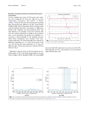
shown in Fig. 7. detected with LOM, while none were detected with OCT,
indicating that the OCT test statistics are less powerful
Illustrated in Fig. 8a and b are the Chi-square test sta- than LOM (for this case).
tistics based on OCT and LOM, respectively. As is seen
from the fgure, all the simulated faults were successfully

Fig. 8 OCT and LOM Chi‑square test statistics for fault detection; equations from (Teunissen 1990) and (Wieser 2004) was adopted; code and
carrier‑phase measurements were processed together to compute these test statistics; P = 0.01
FA