Page 93 - 卫星导航2021年第1-2合期

Shi et al. Satell Navig (2021) 2:5 Page 9 of 13

at 0°
num ) at 125°
at 240°
Percentage of time (≥X

X num

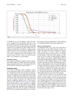
Fig. 8 Percentage of time with the number of visible satellites ≥ X num in scenario 4

0° and 240° are selected for simulation. Tese two orbits form in this section. Te results shown in Table 6 illustrate
can be regarded as the intermediate orbit state of the the contribution of BDS to performance improvement.
spacecraft during the whole orbit maneuver process. Te
orbit elements (RAAN is the right ascension of ascending Number of visible satellites
node) from TLE are listed in the Table 4 (Kelso 2020). To Te simulation results in Fig. 4 show that in the SSTO of
analyze the performances of diferent navigation system launch process (in ECI (Earth-Centered Inertial) coor-
combinations, the results of the physical visibility, PDOP dinates), the single BDS (total 46 satellites) can ofer the
value, received power and the Doppler shift are given similar performance as scenario 2 (total 78 satellites).
in the paper. Furthermore, the C/N 0 threshold of the Compared with scenario 3 and scenario 4, it is obvious
receiver is set as 20 dB·Hz. If the C/N 0 is lower than this that the addition of BDS GEO/IGSO satellites can efec-
value, it will be regarded as invisible signal. tively increase the number of visible satellites. In addition,
in the scenario 4, the number of visible satellites does not
Simulation scenarios always decrease with altitude, except for a few time ranges,
Four scenarios of diferent navigation system combina- the number of visible satellites remains at least 4, which
tions will be utilized to calculate and analyze the auton- provides a guarantee for precise positioning and maneu-
omous navigation performance of the spacecraft in the vering. In this simulation, when the spacecraft height is
SSTO/GEO. Te scenarios are listed in Table 5. lower than 3,000 km, the number of visible satellites will
be reduced to less than 4 because the receiver only has
Simulation results one +Z antenna. Obviously, the visibility performance at
In this part, the simulation results of diferent combina- low attitude can be improved by adding multiple antennas
tions of orbits and scenarios will be presented in steps of e.g., one nadir antenna and one zenith antenna. Te results
60 s. Te SSTO data are the statistical values of 6 orbit peri- with multiple antennas are not discussed in this paper.
ods, and GEO data is in 6 d. In single GNSS, only 4 usable For the spacecraft in GEO at 0°, we can draw the same
satellites are needed for position calculation. Because of the conclusion that the BDS can efectively increase the
inter-system biases, when the satellites from multi-GNSS number of visible satellites. In all four navigation system
are used for position calculation, each additional GNSS combinations, the percentage of the time when the posi-
requires an additional satellite (Liu et al. 2016; Monten- tion is solvable reaches 97% (the percentage of the time
bruck et al. 2018; Odijk et al. 2017). If there are n satellites when usable satellites are 4 or more reaches 100%). How-
from k GNSSs available at time t, only when n–k is greater ever, the number of visible satellites for the spacecraft in
than or equal to 3, the receiver position can be obtained GEO is highly related to its longitude, which can be seen
from the pseudorange measurements. In addition to the from the diference of the number of visible satellites in
percentage of the time when the position is solvable, the the same scenario in Figs. 5 and 6.
PDOP, C/N 0 and Doppler shift will be given in a suitable