Page 191 - 卫星导航2021年第1-2合期

Li et al. Satell Navig (2021) 2:1 Page 5 of 14

c j
where r I (ˆ z b k , χ) and r C (ˆ z , χ) denote the inertial and Te edge between two consecutive nodes is a local con-
b k+1 l straint formed by S-VINS. Another type of edge is the
visual residuals, respectively; r p − H p χ represents the global constraint provided by the multi-GNSS PPP solu-

a priori information obtained by the process of margin- tion. Because of the low satellite availability in complex
alization in the sliding window; ρ(·) is the Huber function driving conditions, the positioning results from the PPP
used for reducing the weight of the outliers in the least are selectively used as the global constraint. A Quality
squares problems (Huber 1964). In addition, a strict out- Number (QN) is adopted to indicate the accuracy of PPP
lier rejection mechanism is performed after each optimi- solution, referring to (NovAtel Corporation 2018a). Te
zation by checking the average reprojection errors of quality of the positioning results from PPP solution are
(13), (14), and (15). When the window size is full, the old- labeled with an integer 1–6 based on their covariances.
est IMU state and corresponding features in the sliding In this paper, the QN within 4 will be maintained in the
window will be marginalized to bound the computational pose graph; the QN equal to 5 will be used only once and
complexity of VIO. removed after the global optimization; and the QN more
Tere are two additional types of reprojection equa-
tions for the stereo VIO compared to the mono-VIO pre- than 5 will be rejected. Te growth rate of the node is
dependent on the GNSS outputs.
sented in Qin et al. (2018). Supposed that the l th feature Te mathematical model of the fusion method can be
is observed by the i th stereo images and the j th stereo expressed as a Maximum Likelihood Estimation (MLE)
images. Additionally, the frst observation of the feature problem as described in Qin et al. (2019). For the com-
happens in the former. Tree types of reprojection equa- pleteness, we briefy introduce the theory. Te state
tions are used in our method, which can be expressed as:

c i,1
1 u
c j,1 c 1 b j w b −1 l b w w b (13)
P = R R w R R π + p + p − p − p
l b b i c 1 c c i,1 c 1 b i b j c 1
l v
l
c i,1
1 u
c j,2 c 2 b j w b −1 l b w w b (14)
P = R R w R R π + p + p − p − p
l b b i c 1 c c i,1 c 1 b i b j c 2
l v
l
c i,1 estimation of the global fusion can be converted to a non-
1 u
c i,2 c 2 b −1 l b b
P = R R π + p − p linear least squares problem, which can be written as:
l b c 1 c c i,1 c 1 c 2
l v
l
n
(15) 2
∗
χ = argmin k k (16)
t
t
c i,1 c i,1 z − h (χ) k
where [u l , v l ] is the frst observation of the lth feature, χ t=0 k∈S � t
and c i,1 denotes the left image of the ith stereo images;
π −1 is the back projection function which turns a pixel where χ=[x 0 , x 1 , . . . x n ] is the state vector of all nodes in
c
G
G
G
G
location into a unit vector using camera intrinsic param- graph and x i =[p , q ] ; p and q are the position and
i i i i
b
b
eters; R , p b and R , p b are the extrinsic parame- orientation of the node i with respect to the global refer-
c 1 c 1 c 2 c 2 ence frame G ; S is the set of measurements including the
ters of left IMU-camera and right IMU-camera,
c j,2
respectively; P and P are the reprojection results local poses (S-VINS) and global positions (multi-GNSS
c j,1
T
l
−1
l
2
from the observations in ith left image to the jth left PPP), Te Mahalanobis norm is �r� k t = r r . Here r
image and right image, respectively; P represents the
c i,2
l
reprojection results from the left image to the right image
in the ith image pair. Te visual measurement residuals
can be obtained by the way of
observed-minus-computed.
Multi‑GNSS PPP/S‑VINS fusion
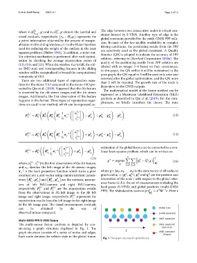
Te multi-sensor fusion problem is depicted by con-
structing a graph structure displayed in Fig. 1. Te
graph structure consists of a series of nodes and edges.
Each node denotes the vehicle state in the global frame.
Fig. 1 The graph structure for global fusion