Page 157 - 卫星导航2021年第1-2合期

Wang et al. Satell Navig (2021) 2:9 Page 7 of 11

(4,−3) (1,−1) (4,−3) (1,−1)
0.5 1.0
RMS = 0.106 RMS = 0.085 0.5
0.0
0.4 GPS FCB bias in cycles −0.5 (1,0) (0,1)
−1.0
1.0
Probability 0.3 −0.5
0.5
0.0
0.2
−1.0
0 4 8 121620240 4 8 12 16 20 24
Time (h)
0.1
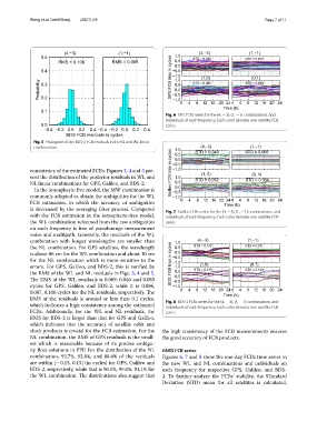
Fig. 6 GPS FCBs series for the (4, − 3), (1, − 1) combinations, and
individuals of each frequency. Each color denotes one satellite FCB
0.0 series
−0.4 −0.2 0.0 0.2 0.4 −0.4 −0.2 0.0 0.2 0.4
BDS FCB residuals in cycles
Fig. 5 Histogram of the BDS-2 FCB residuals in the NL and WL linear
(1,1)
(4,3)
combinations 1.0 STD = 0.049 STD = 0.005
0.5
0.0
−1.0
consistency of the estimated FCBs. Figures 3, 4 and 5 pre- Galileo FCB bias in cycles −0.5 (1, 0)
(0, 1)
sent the distribution of the posterior residuals in WL and 1.0 STD = 0.052 STD = 0.054
NL linear combinations for GPS, Galileo, and BDS-2. 0.5
0.0
In the ionospheric-free model, the MW combination is −0.5
commonly adopted to obtain the ambiguities for the WL −1.0
FCB estimation, in which the accuracy of ambiguities 0 4 8 12162024 0 4 8 12162024
Time (h)
is decreased by the averaging flter process. Compared Fig. 7 Galileo FCBs series for the (4, − 3), (1, − 1) combinations, and
with the FCB estimation in the ionospheric-free model, individuals of each frequency. Each color denotes one satellite FCB
the WL combination reformed from the raw ambiguities series
on each frequency is free of pseudorange measurement
noise and multipath. Generally, the residuals of the WL
combination with longer wavelengths are smaller than 1.0 (4,−3) (1,−1)
the NL combination. For GPS satellites, the wavelength 0.5
is about 86 cm for the WL combination and about 10 cm 0.0
for the NL combination which is more sensitive to the −0.5
−1.0
errors. For GPS, Galileo, and BDS-2, this is verifed by BDS FCB bias in cycles 1.0 (1,0) (0,1)
the RMS of the WL and NL residuals in Figs. 3, 4 and 5. 0.5
0.0
Te RMS of the WL residuals is 0.069, 0.046 and 0.085 −0.5
cycles for GPS, Galileo, and BDS-2, while it is 0.086, −1.0
0.087, 0.106 cycles for the NL residuals, respectively. Te 0 4 8 121620240 4 8 12 16 20 24
Time (h)
RMS of the residuals is around or less than 0.1 cycles,
which indicates a high consistency among the estimated Fig. 8 BDS-2 FCBs series for the (4, − 3), (1, − 1) combinations and
individuals of each frequency. Each color denotes one satellite FCB
FCBs. Additionally, for the WL and NL residuals, the series
RMS for BDS-2 is larger than that for GPS and Galileo,
which indicates that the accuracy of satellite orbit and
clock products is crucial for the FCB estimation. For the the high consistency of the FCB measurements ensures
NL combination, the RMS of GPS residuals is the small- the good accuracy of FCB products.
est which is reasonable because of its precise ambigu-
ity foat solutions in PPP. For the distribution of the NL GNSS FCB series
combination, 92.7%, 92.4%, and 88.4% of the residuals Figures 6, 7 and 8 show the one-day FCBs time series in
are within [− 0.15, 0.15] (in cycles) for GPS, Galileo and the new WL and NL combinations and individuals on
BDS-2, respectively, while that is 96.1%, 99.0%, 91.1% for each frequency for respective GPS, Galileo, and BDS-
the WL combination. Te distributions also suggest that 2. To further analyze the FCBs’ stability, the STandard
Deviation (STD) mean for all satellites is calculated.