Page 278 - 《软件学报》2026年第7期

买宁 等: 高铁复合无线通信信道形式化建模与验证 2963

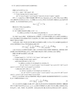
定理 1. 复合信道符合 K 0 分布.
val it : thm = ⊢ sigma1 > &0 /\ sigma2 > &0
==> Product_Rayleigh_Density h sigma1 sigma2 =
(&2 * h) / (power2 sigma1 * power2 sigma2) * Bessel_K0_real (abs h / (sigma1 * sigma2))
定理 1 中, “reallim”来表示实数序列的极限, 即数学符号 lim. “Bessel_K0_real”表示第 2 类修正 Bessel 函数 K 0
分布, 其数学积分形式如公式 (7) 所示. 本文依据公式 (7) 对 K 0 分布进行形式化建模, 以确保其与 p(h) 的最终化简
结果保持一致, 其形式化模型如定义 24 所示.

∫
1 +∞ z 2
K 0 (z) = t e (7)
−1 −t− 4t dt
2 0
定义 24. 第 2 类修正 Bessel 函数 K 0 .
⊢ !z. Bessel_K0_real z =

&1 / &2 * reallim (atreal (&0) within {x | &0 <= x})
(\a. reallim at_posinfinity (\b. real_integral (real_interval [a, b])
(\t. &1 / t * exp (--t + --(power2 z / (&4 * t))))))
第 2 类修正 Bessel 函数是一类在数学物理和工程领域中广泛应用的特殊函数, 其具有多种积分形式和渐近表
达式. 在处理概率分布和无线通信中的复合信道建模时, 第 2 类修正 Bessel 函数的积分形式和渐近性质常被用来
描述信号的长尾分布特性.
为证明定理 1, 需进一步化简并研究复合概率密度函数的分布规律. 在公式 (6) 中代入瑞利概率密度函数公式
并化简, 得到结果如公式 (8), 其形式化描述如定理 2 所示.

∫ h 2 ∫ x h 2
+∞ 1 h 1 − h 2 1 h 1 − h 2
p(h) = lim e − 2σ 2 1 2σ 2 h 2 e − 2σ 2 1 2σ 2 h 2 (8)
2 1 dh 1 + lim
2 1 dh 1
2
2
x→0 + |h 1 | σ σ 2 x→0 − −∞ |h 1 | σ σ 2
x 1 2 1 2
定理 2 对公式 (6)–(8) 的推导过程进行了验证, 其证明过程中需充分考虑复合极限的处理、被积函数不连续
点处理以及积分等价性等问题, 且涉及了大量符号操作和复杂的公式推导, 相对复杂, 此处不做赘述.
定理 2. 复合概率密度函数代入化简定理.
val it : thm =
⊢ !h sigma1 sigma2. h = c * h1 * h2 /\ c = &1 /\ sigma1 > &0 /\ sigma2 > &0
==> Product_Rayleigh_Density h sigma1 sigma2 =
reallim (atreal (&0) within {x | &0 <= x})
(\a. reallim at_posinfinity (\b. real_integral (real_interval [a, b])
(\h1. &1 / abs h1 * h / (power2 sigma1 * power2 sigma2) * exp (--power2 h1 / (&2 * power2
sigma1) + --power2 h / (&2 * power2 sigma2 * power2 h1)))))
+ reallim (atreal (&0) within {x | x <= &0})
(\a. reallim at_neginfinity (\b. real_integral (real_interval [b, a])
(\h1. &1 / abs h1 * h / (power2 sigma1 * power2 sigma2) * exp (--power2 h1 / (&2 * power2
sigma1) + --power2 h / (&2 * power2 sigma2 * power2 h1)))))
此时在公式 (8) 的基础上分析 p(h) 的被积函数, 可验证其为偶函数. 根据偶函数的对称性质对公式 (8) 进行化
简, 进一步得到化简结果如公式 (9).

∫ h 2
+∞ 1 h 1 − h 2
p(h) = 2 lim e − 2σ 2 1 2σ 2 h 2 (9)
2 1 dh 1
2
x→0 + x h 1 σ σ 2 2
1
对公式 (9) 进行形式化建模, 如定理 3 所示. 定理 3 的证明过程需充分考虑被积函数为偶函数这一隐藏前提
∫ b ∫ −b
条件. 其关键在于使用形如 f(x)dx = f(−x)dx 的积分对称性形式化定理. 在使用该定理前, 仍需先经过对证
a −a
明目标重写、化简、实例化、消去相同项等一系列复杂的证明步骤, 将证明目标化简为与积分定理一致的形式.